import os
import sys
ROOT_DIR = os.path.abspath("../../")
# Import Mask RCNN
sys.path.append(ROOT_DIR) # To find local version of the libraryfrom mrcnn.config import Config
from keras import backend as k
from tensorflow.python.framework.graph_util_impl import convert_variables_to_constants
import tensorflow as tf
import mrcnn.model as modellib
classoutConfig(Config):
NAME = "balloon"
NUM_CLASSES = 1 + 1
BACKBONE = "resnet101"
IMAGE_MIN_DIM = 800
IMAGE_MAX_DIM = 1024
GPU_COUNT = 1
IMAGES_PER_GPU = 1
DETECTION_MAX_INSTANCES = 100
MODEL_DIR = os.path.join(ROOT_DIR, "model/balloon/logs") #모델 저장 폴더
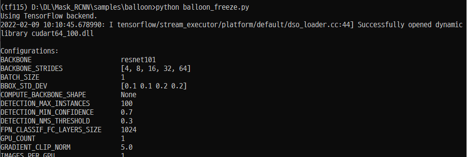
out_config = outConfig()
out_config.display()
model = modellib.MaskRCNN(mode="inference", config=out_config,model_dir=MODEL_DIR)
model_path = model.find_last()
model.load_weights(model_path, by_name=True)
session = k.get_session()
min_graph = convert_variables_to_constants(session,session.graph_def,[out.op.name for out in model.keras_model.outputs])
tf.train.write_graph(min_graph, './', 'mrcnn.pb', as_text=False)
outConfig의 내용은 이전 inference 에서 나왔던 값들과 동일하게 맞춤
(그게 맞는지는 모름 -_-)
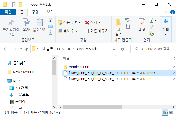
* 실행 성공하면 mrcnn.pb파일이 생성됨
2. 로드 후 테스트 하려면
1) MASK_RCNN/mrcnn/model.py
- MaskRCNN클래스에 다음의 멤버함수를 추가한다
defdetect_pb(self, images, sessd, input_image, input_image_meta, input_anchors, detections, mrcnn_mask, verbose=1):"""Runs the detection pipeline.
images: List of images, potentially of different sizes.
Returns a list of dicts, one dict per image. The dict contains:
rois: [N, (y1, x1, y2, x2)] detection bounding boxes
class_ids: [N] int class IDs
scores: [N] float probability scores for the class IDs
masks: [H, W, N] instance binary masks
"""assert self.mode == "inference", "Create model in inference mode."assertlen(
images) == self.config.BATCH_SIZE, "len(images) must be equal to BATCH_SIZE"# if verbose:# log("Processing {} images".format(len(images)))# for image in images:# log("image", image)# Mold inputs to format expected by the neural network
molded_images, image_metas, windows = self.mold_inputs(images)
#print('molded_images : ', molded_images)#print('image_metas : ', image_metas)#print('windows : ', windows)# Validate image sizes# All images in a batch MUST be of the same size
image_shape = molded_images[0].shape
# print(image_shape, molded_images.shape)for g in molded_images[1:]:
assert g.shape == image_shape,\
"After resizing, all images must have the same size. Check IMAGE_RESIZE_MODE and image sizes."# Anchors
anchors = self.get_anchors(image_shape)
# Duplicate across the batch dimension because Keras requires it# TODO: can this be optimized to avoid duplicating the anchors?
anchors = np.broadcast_to(anchors, (self.config.BATCH_SIZE,) + anchors.shape)
# if verbose:# log("molded_images", molded_images)# log("image_metas", image_metas)# log("anchors", anchors)# Run object detection# detections, _, _, mrcnn_mask, _, _, _ =\# self.keras_model.predict([molded_images, image_metas, anchors], verbose=0)
detectionsed, mrcnn_masked = sessd.run([detections, mrcnn_mask], feed_dict = {input_image: molded_images, \
input_image_meta: image_metas, \
input_anchors: anchors})
print('detectionsed : ', detectionsed.shape)
print('mrcnn_masked : ', mrcnn_masked.shape)
mrcnn_masked = np.expand_dims(mrcnn_masked, 0)
detections = np.array(detectionsed)
mrcnn_mask = np.array(mrcnn_masked)
print('detections : ', detections.shape)
print('mrcnn_mask : ', mrcnn_mask.shape)
# Process detections
results = []
for i, image inenumerate(images):
xi = detections[i]
yi = mrcnn_mask[i]
moldedi = molded_images[i]
windowsi = windows[i]
final_rois, final_class_ids, final_scores, final_masks =\
self.unmold_detections(detections[i], mrcnn_mask[i],
image.shape, molded_images[i].shape,
windows[i])
results.append({
"rois": final_rois,
"class_ids": final_class_ids,
"scores": final_scores,
"masks": final_masks,
})
return results
- filepath: filepath는 (on_epoch_end에서 전달되는) epoch의 값과 logs의 키로 채워진 이름 형식 옵션을 가질 수 있음. 예를 들어 filepath가 weights.{epoch:02d}-{val_loss:.2f}.hdf5라면, 파일 이름에 세대 번호와 검증 손실을 넣어 모델의 체크포인트가 저장 * monitor: 모니터할 지표(loss 또는 평가 지표)
- val_loss : 줄어드는 것을 모니터링
- val_accuracy : 커지는 것을 모니터링 * save_best_only: 가장 좋은 성능을 나타내는 모델만 저장할 여부 * save_weights_only: Weights만 저장할 지 여부
- True : weight와 bias 값만 저장한다
- False : layer 구성, 노드 갯수, 노드 정보, activation 정보 등의 값을 같이 저장한다
- 참고) True를 권장 , SaveWeights / LoadWeights * mode: {auto, min, max} 중 하나. monitor 지표가 감소해야 좋을 경우 min, 증가해야 좋을 경우 max, auto는 monitor 이름에서 자동으로 유추.
- monitor가 val_loss인 경우 min
- monitor가 val_accuracy인 경우 max
* period 확인 횟수 : 1이면 매번 1epoch시 확인, 3이면 3epoch시 확인
from tensorflow.keras.callbacks import ModelCheckpoint
from tensorflow.keras.optimizers import Adam

model = create_model()
model.compile(optimizer=Adam(0.001), loss='categorical_crossentropy', metrics=['accuracy'])

mcp_cb = ModelCheckpoint(filepath='/kaggle/working/weights.{epoch:02d}-{val_loss:.2f}.hdf5', monitor='val_loss',
                         save_best_only=True, save_weights_only=True, mode='min', period=3, verbose=1)
history = model.fit(x=tr_images, y=tr_oh_labels, batch_size=128, epochs=10, validation_data=(val_images, val_oh_labels),
                   callbacks=[mcp_cb])
2.ReduceLROnPlateau(monitor='val_loss', factor=0.1, patience=10, verbose=0, mode='auto', min_delta=0.0001, cooldown=0, min_lr=0) * 특정 epochs 횟수동안 성능이 개선 되지 않을 시 Learning rate를 동적으로 감소 시킴 * monitor: 모니터할 지표(loss 또는 평가 지표) * factor: 학습 속도를 줄일 인수. new_lr = lr * factor * patience: Learing Rate를 줄이기 전에 monitor할 epochs 횟수. * mode: {auto, min, max} 중 하나. monitor 지표가 감소해야 좋을 경우 min, 증가해야 좋을 경우 max, auto는 monitor 이름에서 유추.
3. EarlyStopping(monitor='val_loss', min_delta=0, patience=0, verbose=0, mode='auto', baseline=None, restore_best_weights=False) 특정 epochs 동안 성능이 개선되지 않을 시 학습을 조기에 중단 monitor: 모니터할 지표(loss 또는 평가 지표) patience: Early Stopping 적용 전에 monitor할 epochs 횟수. mode: {auto, min, max} 중 하나. monitor 지표가 감소해야 좋을 경우 min, 증가해야 좋을 경우 max, auto는 monitor 이름에서 유추.
* 예를 들어 loss는 계속 줄어드는데, val_loss는 늘어나는 경우
from tensorflow.keras.callbacks import EarlyStopping

model = create_model()
model.compile(optimizer=Adam(0.001), loss='categorical_crossentropy', metrics=['accuracy'])

ely_cb = EarlyStopping(monitor='val_loss', patience=3, mode='min', verbose=1)
history = model.fit(x=tr_images, y=tr_oh_labels, batch_size=128, epochs=30, validation_data=(val_images, val_oh_labels),
                   callbacks=[ely_cb])
1-3) 모델 컴파일(전에 어디서 들었을 때는 생성된 노드들 조립하는 과정이라고 들었는데 맞는지는...????)
- 분류 모델이므로 categorical_crossentropy
from tensorflow.keras.optimizers import Adam
from tensorflow.keras.losses import CategoricalCrossentropy
from tensorflow.keras.metrics import Accuracy

model.compile(optimizer=Adam(0.001), loss='categorical_crossentropy', metrics=['accuracy'])
#who 명령 : 메모리 상의 변수#load 함수 : 데이터 파일을 읽어들임, 변수명은 파일명으로
load('featureX.dat') # featureX 변수에 할당됨#whos 명령 : 메모리 상의 변수와 상세 정보등을 보여줌(Name, Size, Bytes, Class)#clear featureX : 메모리상에서 featureX 변수 제거
V = featuresX(1:10) #features 처음 10개의 데이터를 V에 저장
save hello.mat V; #V 변수의 데이터를 hello.mat파일에 저장
clear #모든 변수를 다 지움
load hello.mat #V 변수가 다시 생김
save hello.txt V -ascii#텍스트로 저장